How to Read a Cardiac MRI

• Open cvi42 application

• On left pane ‘Viewer’ is your homebase

• 3 groups of MRI images (in order)

  • Echo-like images

• Flow

  • On Left pane select, Flow 2D
  • Select flow images → drag them in
  • See Total Forward Volume, Total Backward Volume, etc.
  • Load aortic and pulmonary flows → Click ‘Comparison’ → Will automatically calculate a Qp/Qs for you

• MPR View

  • Only works with certain sequences

• 4D flow is free breathing

  • We use Arterys (now under Tempus)
  • Can use to calculate Qp/Qs as well

• tiscout to pick where myocardium is darkest/blackest. ti-scout to identify the time when the myocardium is nulled

  • Amyloid never nulls
  • “Normal myocardial nulling argues against Amyloidosis”
  • Phase-sensitive inversion recovery (PSIR) lets the computer try to figure it out. Try if can’t null and see if computer can figure it out.

Buttonology

• Shift+Right click for window/level
• Alt+R to rotate images
  • Orme used this to get anterior wall on SAX at 12 o’clock

Viewer

Scout Images

• Start reading your scout images and assess extra-cardiac findings

t1 vibe dixon

• The POST t1 vibe dixon has been described to me as the “poor man’s CTA”
• Useful for making measurements of aorta, look at pulmonary veins, etc.
• Measure the main PA at bifurcation on vibe view.
  • Think pulmonary HTN if > 30 mm
• Dr. Saghir also uses this to examine extra-cardiac findings

Steady State Free Precession (SSFP)

• SSFP images exhibit T1 and T2 weighting and is portrayed in cine mode
• SSFP offers a very high signal-to-noise ratio and a T2/T1-weighted image contrast.¹
• trufi sequence on Siemens provides a good contrast b/w blood pool, which appears bright 🔆, and the myocardium
  • Gated images
• SSFP goes by different names depending on the vendor:
  • Siemens: TRUFI (true fast imaging with steady-state precession)
    • generally believed to exhibit T2 /T1-weighting
  • GE: FIESTA (Fast Imaging Employing Steady-state Acquisition)
  • Philips: Balanced-FFE (Fast Field Echo)

Thrombus Detection

“High TI” is your thrombus hunter.

• Dr. Saghir

• In Viewer, load your “high TI” images, e.g. Post 4Ch stack high TI *
• High TI imaging is great to see clot/thrombus, which will appear dark/black ⚫
• High TI images (e.g. TI of 600) are very useful to look for thrombus.
  • Very good for LV apical thrombus.
• These images do not have the spatial resolution to r/o LAA thrombus, so you cannot exclude the possibility of LAA thrombus if not visualized.

PSIR

• PSIR stands for Phase-sensitive inversion recovery
• Immediate post-contrast images
  • Shortly after the administration of contrast agents, PSIR can be used to enhance the visualization of vascular structures and myocardial perfusion. The immediate phase primarily benefits from the high contrast provided by gadolinium-based contrast agents circulating in the bloodstream. Immediate post-contrast PSIR sequences are mainly used for the visualization of clots and tumors. (Source)
• Delayed post-contrast images to look for Late Late Gadolinium Enhancement (LGE)
  • Selection of TI time (Source)
    • the inversion time (TI) is critically selected to nullify the signal from the normal myocardium.
    • TI is often determined by a Look-Locker sequence .
    • By setting the TI such that the normal myocardium’s signal is zero (nulled), any remaining enhanced regions (indicative of fibrosis or scar tissue) are conspicuously bright against the dark background of the healthy myocardial tissue.
  • In our lab, 10 minutes post-contrast they do another scout. It is on this series, they will look for “nulling.” In other words, the scout images are used to determine a TI time. Using this TI time, another series of images will be obtained.
    • By the 10 minute mark, the gadolinium should have washed out.
    • Dr. Saghir likes to compare these to the 4CH acquired at the beginning of the study.
  • MOCO means motion correction
    • MOCO is most useful with the LGE stacks b/c that it when you most often get artifact.

Absence of "nulling" → think Amyloidosis

The absence of nulling suggests cardiac amyloidosis.

Measure LV wall thickness

• Dr. Saghir likes to do this in the Function SAX module in Circle.
• Measuring LV wall thickness using a SAX stack. It should be done at the thickest portion. According to Dr. Saghir, it is most commonly (“9 times out of 10”) thickest in the basal septum.

T1 weighted images

• T1 is “just a hydrogen detector”

T2 weighted images

• On the Siemens scanner, you will see these as SAX HASTE series
• Scroll through these images to see if anything is lighting up
  • For example, we saw a large pericardial effusion that was bright and this sequence told us that it was just fluid filled.

T2* mapping

• On the left panel, select Tissue T2* Mapping → drag the sax_t2starmap_ image series in
• Use the freehand drawing tools on the top panel, i.e. 1, 2, to draw areas within the septum to quantify iron deposition in the heart 🫀 and within the liver.
• Visually, you will also want to note if each organ appears blacker 🖤 than expected, which would also suggest iron overload.

Function SAX: Measure ventricle size and EF

• On the left panel, select Function SAX
• Pull in cine_trufi_* SAX stack
• Pull in cross reference views in the smaller two windows to the right
• Find diastole (and systole) to correspond to your measurements of interest
• Click the ⭕ button on the top panel to draw the LV endocardial contour at each slice
  • With your mouse, hold down Alt and move your mouse to do the tracing
  • If you need to adjust the tracing after, just left-click on your mouse 🖱️ and adjust the border
  • You can always undo by clicking Ctrl+Z
• For tracing the RV, click the yellow half-circle button on the top panel

Lining up systolic and diastolic tracings

Generally, systolic should start tracing 1 or so level below the diastolic tracing. In folks with very sick hearts, can be at the same level.

• SV should be between LV and RV should be +/- 10 mL
  • not accounting for regurgitation, etc.

Function Biplanar LAX

• The Function Biplanar LAX module can auto-calculate stuff for you.
• Pull in your trufi 2CH and trufi 4CH into the corresponding regions → On the top panel, click the first auto-contour button (denoted with a ⭐) that is Segment LAX Endo

MPR

• Can click MPR and drag the t1 vibe dixon image in there to measure aortic dimensions

Flow 2D

• Use this module to quantify using both aortic and pulmonic AA flow * image stacks
  • You get two for each (i.e. aortic and PA) — calculate and average for each of them.
• Flow 2D is done with all non-contrast images.
  • By contrast, Arterys requires gadolinium enhanced images
• For quality control, visually inspect the images for evidence of aliasing

Reference Ranges

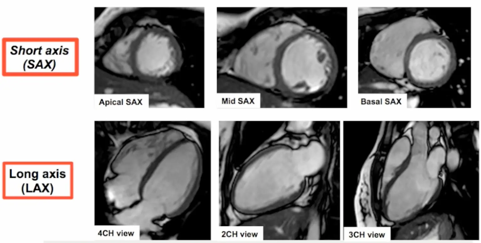
Left Ventricle

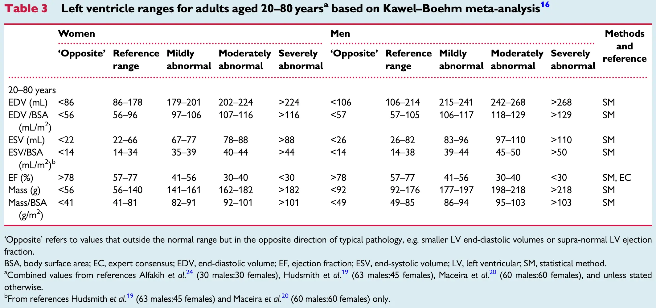Table source: ²

Right Ventricle

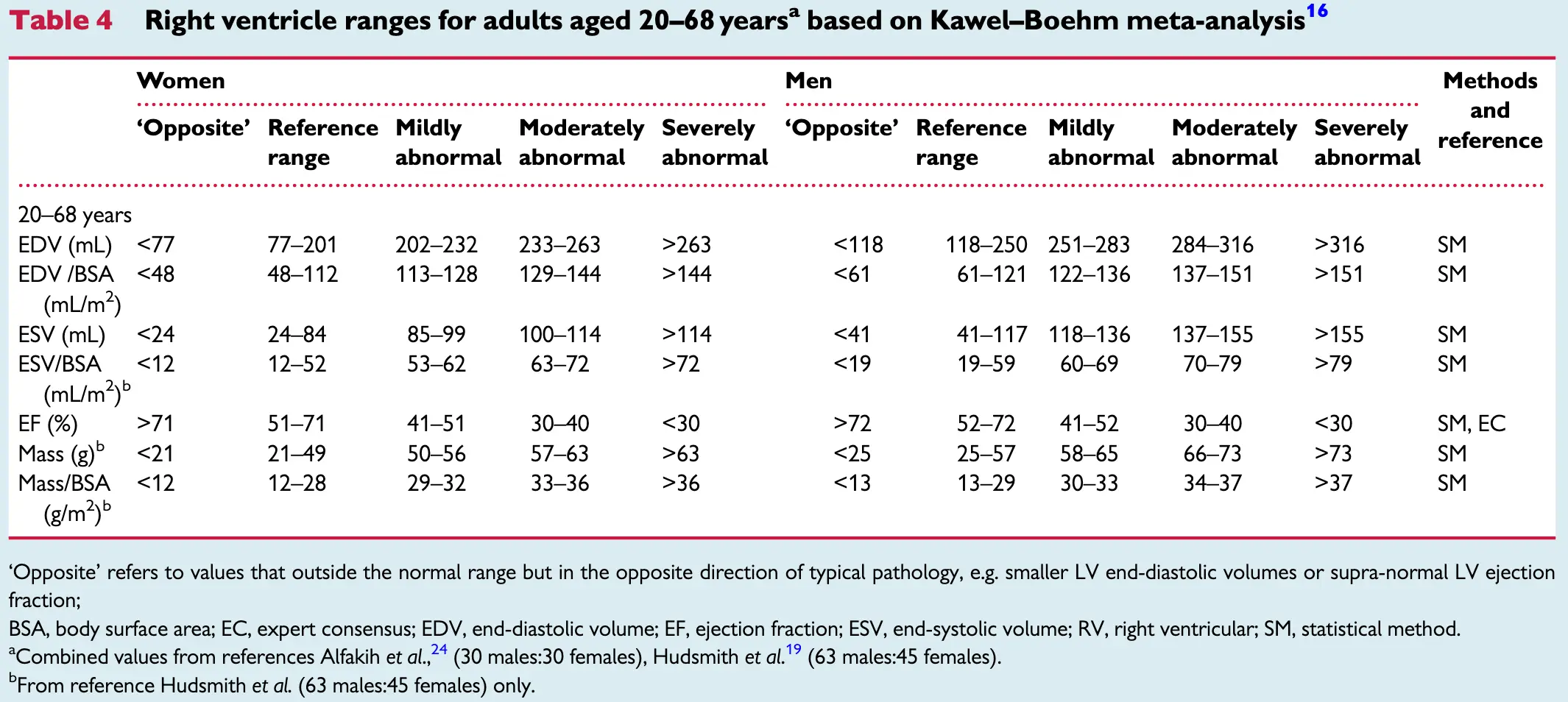Table source: ²

Valve Regurgitation

Mitral and tricuspid regurgitation

	Mild	Moderate	Severe
Regurgitant fraction (%)	0-20	21-40	>40
Regurgitant volume (mL/cycle)	0-30	31-60	>60
AR LV end-diastolic volume index (mL/m2)			>100

Aortic and pulmonary regurgitation

	Mild	Moderate	Severe
Regurgitant fraction (%)	0-15	16-30	>30
Regurgitant volume (mL/cycle)	0-20	21-40	>40
AR LV end-diastolic volume index (mL/m2)			>130

Basic Cardiac Views

How CMR Images Are Obtained

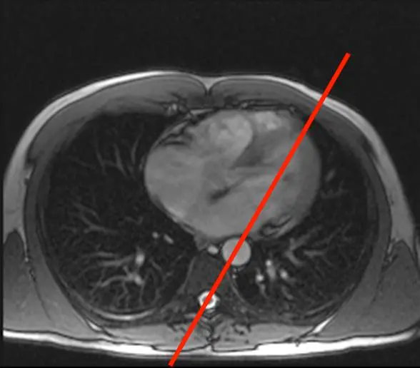
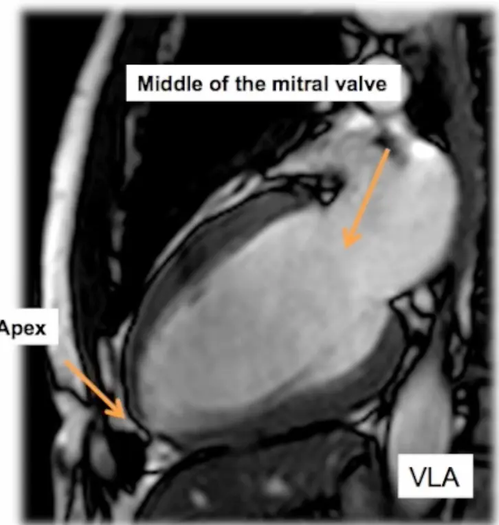
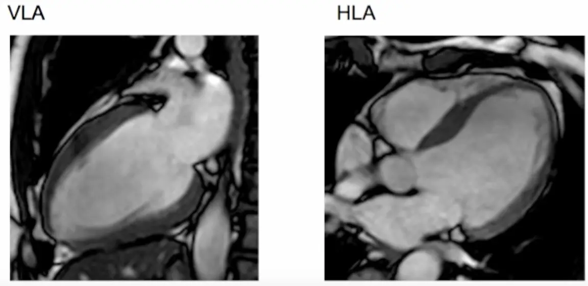
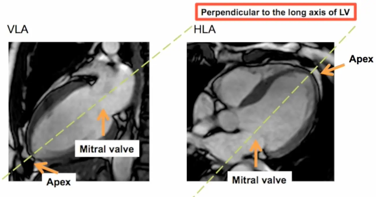
• Step 1. Scouts and planning views (VLA, HLA)
  • We begin with the transverse LAX view and position the line marker dissecting the apex and the middle of the mitral valve (where the two leaflets meet) → results in a vertical LAX (VLA) view, aka pseudo 2 chamber (p2CH) view
    • 
    • 
  • Next we slice the resulting VLA view: again, we cut across the apex and the middle of the mitral valve (where the two leaflets meet) → results in a horizontal LAX (HLA) view
    • 
  • Resulting scout views include VLA and HLA views
    • 
• Step 2. Short axis (SAX) stack acquisition
  • The SAX stack is acquired using cuts that are perpendicular to the VLA and HLA views. The SAX stack acquisition has the advantage of minimizing oblique cuts through the myocardium, which may provide a false impression of regional wma.
    • 
  • 5-slice LV slicing is conducted using end-systole
• Step 3. Long axis (LAX) views acquisition
  • 4CH view
  • 3CH view
  • 2CH view

Footnotes

1. Bieri O, Scheffler K. Fundamentals of balanced steady state free precession MRI. J Magn Reson Imaging 2013;38:2-11. ↩

2. Steffen E Petersen, Mohammed Y Khanji, Sven Plein, Patrizio Lancellotti, Chiara Bucciarelli-Ducci, European Association of Cardiovascular Imaging expert consensus paper: a comprehensive review of cardiovascular magnetic resonance normal values of cardiac chamber size and aortic root in adults and recommendations for grading severity, European Heart Journal - Cardiovascular Imaging, Volume 20, Issue 12, December 2019, Pages 1321–1331, https://doi.org/10.1093/ehjci/jez232 ↩ ↩²