- Cardiac MRI are usually done on 1.5 Tesla (30,000 times the Earth’s magnetic field)
- ⚠️ Safety issue: the magnet 🧲 is always on
- In the presence of a strong magnetic field (typically 0.5 – 3.0 Tesla (T) for clinical applications) atoms ⚛︎ in the body (typically hydrogen) are stimulated to emit radio waves 🔊. These radio waves 🔊 are detected by an antenna (more specifically, the radiofrequency coils) placed around, or over, the body part of interest allowing an image of the body to be reconstructed.
- Extra magnetic fields (using gradient coils) are used to constantly change the magnetic field to allow images of the body to be reconstructed.
- The typical magnetic field strengths used in clinical MRI scanners are:
- 1.5 Tesla
- 3 Tesla
- Excitation: The RF pulse (radiowave) causes a proton to be excited → flips from low- to high-energy state
- Relaxation
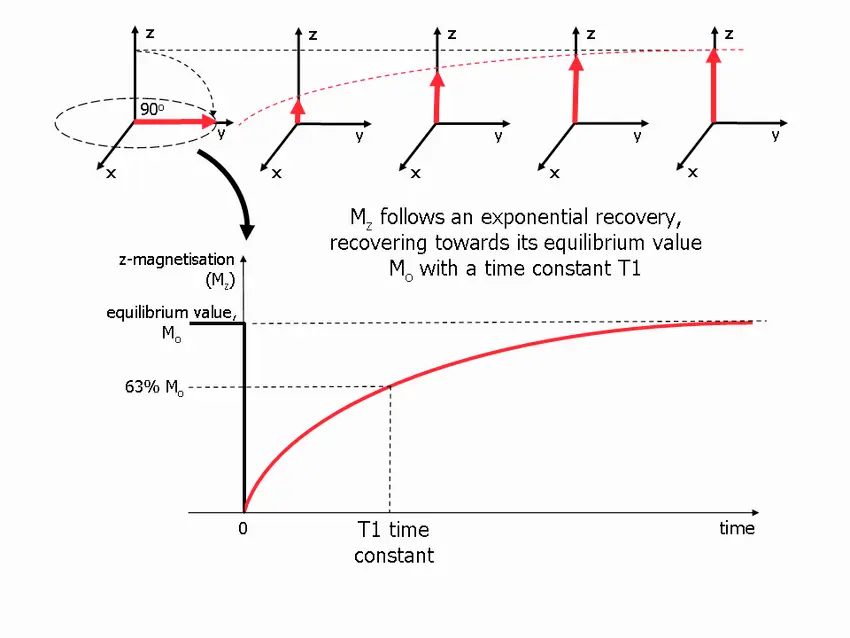
- T1 Recovery
- the natural tendency is to from high-energy state back to a low-energy state
- there is a predictable rate of regrowth/relaxation.
- In the figure below, you are going from the high-energy state in the transverse plane () where the flip angle is 90˚ (100% transverse magnetization and 0% longitudinal magnetization) and there is “regrowth” towards the low-energy state where the flip angle is 0˚ in the longitudinal axis () and the protons are aligned upright in the direction of the main magnetic field.
- When this rate of regrowth is mapped over time, the T1 time constant is the amount of time it takes to regain 63% of the intrinsic (full) magnetization ()
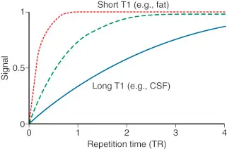
- 📝 T1 time is tissue-specific, i.e. different tissues have different T1 times
- Fat has short T1 times, i.e. hydrogen protons that are within fat will have very fast T1 recovery
- ~200-250 ms
- Water has very slow T1 recovery times
- ~2,000 ms (10-fold greater T1 relaxation time compared to fat❗)
- Fat has short T1 times, i.e. hydrogen protons that are within fat will have very fast T1 recovery
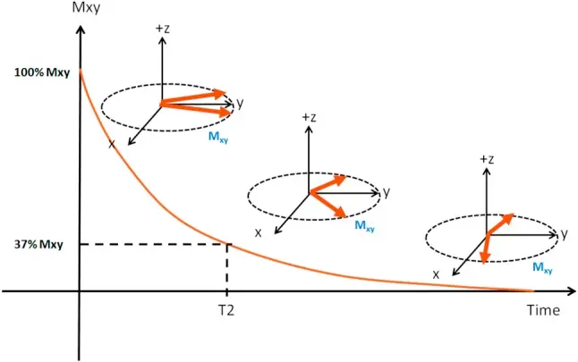
- T2 Decay (aka spin-spin relaxation)
- When the RF excitation pulse is applied, the protons are all spinning in-phase. Immediately after this pulse is applied, they begin to dephase at a rate proportional to the amount of the magnetic field → eventually, protons will return to their out-of-phase initial pre-RF excitation state, as measured by the T2 relaxation time. (Source)
- The rate of dephasing is different for each tissue, resulting in further tissue contrast.
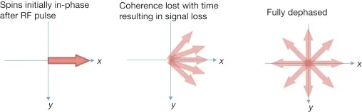
- 📝 this “dephasing” is occurring in the -plane
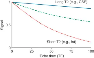
- T2 decay time is the amount of time it takes to drop your magnetization to 37% of what it was after you first applied a 90˚ RF pulse.
- T2 decay time is tissue-specific
- Fat: T2 decay time is fast 🏎️ at 84 ms
- Water: T2 decay time is longer (~1400 ms)
- T1 Recovery
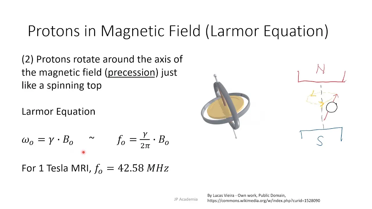
- The Larmor equation is a mathematical formula that describes the precession frequency of nuclei in a substance placed in a static magnetic field
- used to calculate the frequency of an RF signal that causes a change in the nucleus spin energy level.
- : the gyromagnetic ratio is different for each nucleus of different atoms.
- : the stronger the magnetic field (), the higher the precessional frequency ().
- (instead of , also applies to , )
- At 1.5T, the protons are spinning around 64 MHz
- At 3T, protons are spinning around at 128 MHz
Earth's 🌎 magnetic field 🧲
The Earth’s magnetic field, which is typically around 25-65 microtesla (µT). Therefore, 1 Tesla is about 30,000 times the earth’s magnetic field.
MRI Machine
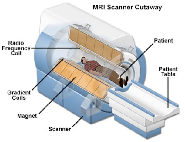
- Layers of the MRI scanner coils (listed from outer-to-inner)
- Main magnet coils ()
- defines the strength of the constant magnetic field (), which is typically measured in Tesla units.
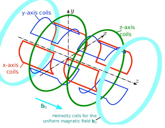
- Gradient coils ()
- Series of coils within main magnet
- 3 sets: , , and directions
- The -axis is parallel to
- 3 sets: , , and directions
- Make slight alterations to the local magnetic field in a graded fashion
- e.g. consider the gradient along the -axis. At some portion of the body (let’s say the middle of the body), the magnetic field strength is at isocenter (1.5 in a 1.5T scanner, 3 in a 3T scanner) and moving towards the head may be 1.51, 1.52, etc. (∴ precession frequency will be higher towards the head) and towards the feet may be 1.49, 1.48, etc. ( will be lower moving towards the feet)
- Units are measured in milliTesla/meter (mT/m)
- Can be turned on/off
- Allow for spatial localization given the coordinate axis reference system afforded by the , , and axes. ∴, allows you to register all of your images b/c you are in a fixed coordinate system.
- Safety issues:
- Loud noise
- make the familiar banging sounds of an MRI scan
- Peripheral nerve stimulation - temporary
- Loud noise
- Series of coils within main magnet
- Radiofrequency coils ()
- Innermost layer of coils
- There are 2 sets of RF coils:
- transmitter coils
- send in a RF pulse → excitation of protons
- generally located within the MRI scanner itself
- receiver coils
- receive radiowaves → signal is processed to generate your image
- typically flexible coils places around the patient; best quality if they are as close as possible to the area you’re trying to image
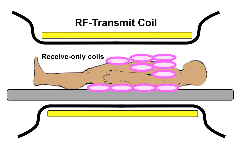
- transmitter coils
- Turn on/off
- Help generate MRI image
- Safety issues:
- Burns
- Device malfunction
- Main magnet coils ()
Terminology
| Term | Meaning |
|---|---|
| T1 [ms] | Time constant representing the recovery of longitudinal magnetization (spin-lattice relaxation) |
| Native T1 | T1 in the absence of an exogenous contrast agent |
| T2 [ms] | Time constant representing the decay of transverse magnetization (spin-spin relaxation) |
| T2* [ms] | Time constant representing the decay of transverse magnetization in the presence of local field inhomogeneities |
| ECV [%] | Extracellular volume fraction, calculated by where myo = myocardium; blood = intracavitary blood pool; Hct = cellular volume fraction of blood [%] |
| Synthetic ECV [%] | ECV where hematocrit is not measured by laboratory blood sampling but derived from blood T1 |
| Parametric mapping | A process where a secondary image is generated in which each pixel represents a specific magnetic tissue property (T1, T2, or T2*) or a derivative such as ECV) derived from the spatially corresponding voxel of a set of co-registered magnetic resonance source images |
FAQs
- Is my patient too big for a Cardiac MRI?
- Table weight limit is 400 lbs, but distribution of weight is the more important feature.
- Wide bore MRI scanners can help
Note
There is no “open MRI” for Cardiac MRI.
- Is my patient’s kidney function too poor for a Cardiac MRI?
- Lot of Cardiac MRI scans don’t require contrast
- We do need contrast for late-gadolinium enhancement
- Nephrogenic Systemic Fibrosis
- first described in HD patients in the late 90s; NSF d/t systemic manifestations
- Avoid gadolinium in patients with poor renal function: severe renal disease (eGFR <30 mL/min/1.73 m.2)
- Some exceptions are made with shared decision making, patient consent
- Newer agents (macrocyclic agents) should be fine w/ poor renal function(?)
- Compared to older (linear) agents
- Can I order a Cardiac MRI if my patient has a device (e.g. pacemaker, ICD)?
- If pt is pacemaker dependent, MRI may suppress the function of the pacemaker. Thus, some adjustments may be needed prior to the MRI.
- If ICD, Cardiac MRI could make device think pt in VT → inadvertent shock!
- Can I order Cardiac MRI on a pregnant 🤰 or lactating woman 🤱?
- Gadolinium is potentially teratogenic
- Gadolinium does go into the breastmilk for 24-48 hrs, so can “pump and dump”
- How can I learn how to do Cardiac MRI?
- Combined Cardiac MRI/CT rotation
- When should I order a Cardiac MRI?
- NICM
- Amyloid, Sarcoid, Iron overload, Fabry’s, Non-compaction
- Adult Congenital Heart Disease
- Hypertrophic Cardiomyopathy
- Echo better at detecting peak LVOT gradient, but MRI better at wall thickness, late gadolinium enhancement, LV apical aneurysm
- Arrhythmia w/u: assess for ARVC, Sarcoid
- r/o LV thrombus
- Pulmonary/AV regurgitation
- NICM